4.2 Complete Neural network

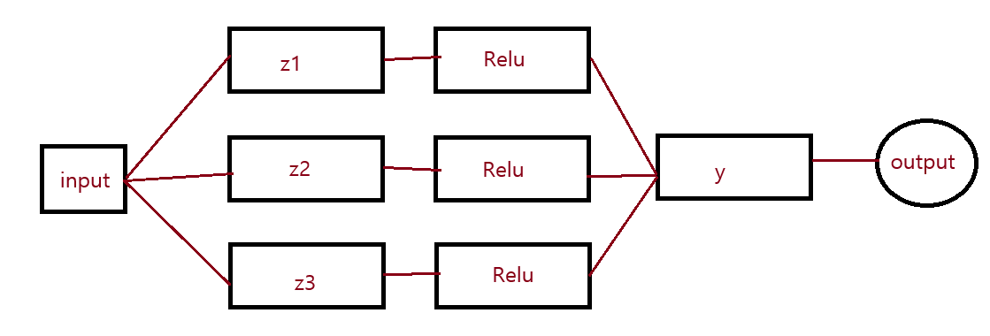The complete training loop is:

INPUT
  ↓
FORWARD PASS
  ↓
LOSS
  ↓
BACKPROPAGATION
  ↓
GRADIENTS
  ↓
UPDATE WEIGHTS AND BIASES
  ↓
NEXT TRAINING STEP

---

2. Forward Pass

We have two inputs:

input	target
$x=\begin{bmatrix}x_1=2\\x_2=3\end{bmatrix}$	20

Hidden Layer

Three neurons:

inputs/targets	neurons	weights	bias	Relu	Loss
	$z_1=w_{11}x_1+w_{12}x_2+b_1$	w11 = 1 w12 = 2	1	$a_1=ReLU(z_1)$	$\boxed{L=(target-y)^2}$
x1=2	$z_2=w_{21}x_1+w_{22}x_2+b_2$	w21 = 2 w22 = 1	2	$a_2=ReLU(z_2)$
x2=3	$z_3=w_{31}x_1+w_{32}x_2+b_3$	w31 = 1 w32 = 1	1	$a_3=ReLU(z_3)$
target=20	$y=w_1a_1+w_2a_2+w_3a_3+b$	w1 = 1 w2 = 2 w3 = 1	1

---

3.1 Forward Pass

First hidden neuron:

$$z_1=(1)(2)+(2)(3)+1$$ $$z_1=9$$

Second:

$$z_2=(2)(2)+(1)(3)+2$$ $$z_2=9$$

Third:

$$z_3=(1)(2)+(1)(3)+1$$ $$z_3=6$$

All are positive, so ReLU does nothing:

$$a_1=9,\quad a_2=9,\quad a_3=6$$

Final neuron:

$$y=(1)(9)+(2)(9)+(1)(6)+1$$ $$y=34$$

Loss:

$$L=(20-34)^2$$ $$\boxed{L=196}$$

---

4. Backpropagation

Backpropagation means calculating:

$$\boxed{\frac{dL}{d\text{parameter}}}$$

for every weight and bias.

We start at the loss and move backward.

L
↓
y
↓
a1, a2, a3
↓
z1, z2, z3
↓
hidden weights and biases

The chain rule is the main mechanism.

---

5. Start at the Loss

Our loss is:

$$L=(target-y)^2$$

Therefore:

$$\frac{dL}{dy} = -2(target-y)$$

Here:

$$target=20$$

and:

$$y=34$$

So:

$$\frac{dL}{dy} = -2(20-34)$$ $$\boxed{\frac{dL}{dy}=28}$$

The positive gradient tells us that increasing the prediction increases the loss at this point.

---

10. All Gradients

We have now backpropagated through the entire network.

Hidden layer

$$\frac{dL}{dw_{11}}=56$$ $$\frac{dL}{dw_{12}}=84$$ $$\frac{dL}{db_1}=28$$ $$\frac{dL}{dw_{21}}=112$$ $$\frac{dL}{dw_{22}}=168$$ $$\frac{dL}{db_2}=56$$ $$\frac{dL}{dw_{31}}=56$$ $$\frac{dL}{dw_{32}}=84$$ $$\frac{dL}{db_3}=28$$

Final neuron

$$\frac{dL}{dw_1}=252$$ $$\frac{dL}{dw_2}=252$$ $$\frac{dL}{dw_3}=168$$ $$\frac{dL}{db}=28$$

Every trainable parameter now has a gradient.

---

11. Weight and Bias Update

Backpropagation gave us the gradients.

Now gradient descent uses them to change the parameters.

The update rule is:

$$\boxed{ parameter_{new} = parameter_{old} - \eta \frac{dL}{d(parameter)} }$$

where $\eta$ is the learning rate.

Use:

learning_rate = 0.001

For example:

$$w_1^{new} = 1-0.001(252)$$ $$\boxed{w_1^{new}=0.748}$$

For $w_2$:

$$w_2^{new}=2-0.001(252)$$ $$\boxed{w_2^{new}=1.748}$$

For $b$:

$$b^{new}=1-0.001(28)$$ $$\boxed{b^{new}=0.972}$$

The same update is performed for every parameter.

---

12. Complete Training Step in Python

Here is the entire process without [PyTorch](../../Course-1-Mathematics and Frameworks/Ch-9 Deep-Learning-Frameworks/PyTorch.mdx).

import numpy as np


# -------------------------
# Data
# -------------------------

x = np.array([2.0, 3.0])
target = 20.0


# -------------------------
# Parameters
# -------------------------

W = np.array([
    [1.0, 2.0],
    [2.0, 1.0],
    [1.0, 1.0]
])

b_hidden = np.array([1.0, 2.0, 1.0])

w_output = np.array([1.0, 2.0, 1.0])
b_output = 1.0

learning_rate = 0.001


# -------------------------
# Forward pass
# -------------------------

z = W @ x + b_hidden

a = np.maximum(0, z)

y = w_output @ a + b_output

loss = (target - y) ** 2


# -------------------------
# Backpropagation
# -------------------------

# Loss -> output
dL_dy = -2 * (target - y)


# Output neuron
dL_dw_output = dL_dy * a
dL_db_output = dL_dy

# Gradient flowing into hidden activations
dL_da = dL_dy * w_output


# ReLU
d_relu = (z > 0).astype(float)

dL_dz = dL_da * d_relu


# Hidden layer
dL_dW = np.outer(dL_dz, x)
dL_db_hidden = dL_dz


# -------------------------
# Parameter updates
# -------------------------

W -= learning_rate * dL_dW
b_hidden -= learning_rate * dL_db_hidden

w_output -= learning_rate * dL_dw_output
b_output -= learning_rate * dL_db_output


# -------------------------
# Results
# -------------------------

print("prediction:", y)
print("loss:", loss)

print("dL/dW:")
print(dL_dW)

print("dL/db_hidden:")
print(dL_db_hidden)

print("dL/dw_output:")
print(dL_dw_output)

print("dL/db_output:")
print(dL_db_output)

print("updated W:")
print(W)

print("updated hidden bias:")
print(b_hidden)

print("updated output weights:")
print(w_output)

print("updated output bias:")
print(b_output)

---

13. Training for Multiple Steps

One training step only changes the parameters once.

Training means repeating:

forward
→ loss
→ backward
→ update
→ forward
→ loss
→ backward
→ update
→ ...

Example:

for step in range(1000):

    # Forward
    z = W @ x + b_hidden
    a = np.maximum(0, z)
    y = w_output @ a + b_output

    # Loss
    loss = (target - y) ** 2

    # Backpropagation
    dL_dy = -2 * (target - y)

    dL_dw_output = dL_dy * a
    dL_db_output = dL_dy

    dL_da = dL_dy * w_output

    d_relu = (z > 0).astype(float)
    dL_dz = dL_da * d_relu

    dL_dW = np.outer(dL_dz, x)
    dL_db_hidden = dL_dz

    # Update
    W -= learning_rate * dL_dW
    b_hidden -= learning_rate * dL_db_hidden

    w_output -= learning_rate * dL_dw_output
    b_output -= learning_rate * dL_db_output

    if step % 100 == 0:
        print(step, y, loss)

The important distinction is:

$$\boxed{\text{Backpropagation} \rightarrow \text{calculate gradients}}$$ $$\boxed{\text{Gradient Descent} \rightarrow \text{update parameters}}$$

Together:

$$\boxed{ Forward \rightarrow Loss \rightarrow Backpropagation \rightarrow Gradient\ Descent \rightarrow Repeat }$$

This is the complete training process for our master network.