4.2. Backpropagate Through the Final Neuron

4. Backpropagation

Backpropagation means calculating:

$$\boxed{\frac{dL}{d\text{parameter}}}$$

for every weight and bias.

We start at the loss and move backward.

L
↓
y
↓
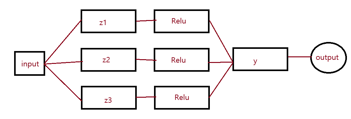
a1, a2, a3
↓
z1, z2, z3
↓
hidden weights and biases

The chain rule is the main mechanism.

---

5. Start at the Loss

Our loss is:

$$L=(target-y)^2$$

Therefore:

$$\frac{dL}{dy} = -2(target-y)$$

Here:

$$target=20$$

and:

$$y=34$$

So:

$$\frac{dL}{dy} = -2(20-34)$$ $$\boxed{\frac{dL}{dy}=28}$$

The positive gradient tells us that increasing the prediction increases the loss at this point. The final neuron is:

$$y=w_1a_1+w_2a_2+w_3a_3+b$$

We need gradients for:

$$w_1,w_2,w_3,b$$

Gradient of w1

$$\frac{dy}{dw_1}=a_1$$

Therefore:

$$\frac{dL}{dw_1} = \frac{dL}{dy} \frac{dy}{dw_1}$$ $$=28(9)$$ $$\boxed{\frac{dL}{dw_1}=252}$$

Gradient of w2

$$\frac{dL}{dw_2} = \frac{dL}{dy}a_2$$ $$=28(9)$$ $$\boxed{\frac{dL}{dw_2}=252}$$

Gradient of w3

$$\frac{dL}{dw_3} = \frac{dL}{dy}a_3$$ $$=28(6)$$ $$\boxed{\frac{dL}{dw_3}=168}$$

Gradient of final bias

Because:

$$\frac{dy}{db}=1$$

we get:

$$\boxed{\frac{dL}{db}=28}$$

---

7. Continue Backward Through the Hidden Layer

Now we need gradients for:

$$a_1,a_2,a_3$$

For $a_1$:

$$\frac{dy}{da_1}=w_1$$

Therefore:

$$\frac{dL}{da_1} = \frac{dL}{dy} \frac{dy}{da_1}$$ $$=28(1)$$ $$\boxed{\frac{dL}{da_1}=28}$$

For $a_2$:

$$\frac{dL}{da_2}=28(2)$$ $$\boxed{\frac{dL}{da_2}=56}$$

For $a_3$:

$$\frac{dL}{da_3}=28(1)$$ $$\boxed{\frac{dL}{da_3}=28}$$

---

8. Backpropagate Through ReLU

ReLU is:

$$a=ReLU(z)=\max(0,z)$$

Its derivative is:

$$\frac{da}{dz} = \begin{cases} 1 & z>0\\ 0 & z<0 \end{cases}$$

Our values are:

$$z_1=9,\quad z_2=9,\quad z_3=6$$

All are positive.

Therefore:

$$\frac{da_1}{dz_1}=1$$ $$\frac{da_2}{dz_2}=1$$ $$\frac{da_3}{dz_3}=1$$

So:

$$\frac{dL}{dz_1} = \frac{dL}{da_1} \frac{da_1}{dz_1} = 28(1) = 28$$ $$\boxed{\frac{dL}{dz_1}=28}$$

Similarly:

$$\boxed{\frac{dL}{dz_2}=56}$$ $$\boxed{\frac{dL}{dz_3}=28}$$

---

9. Backpropagate Into Hidden Weights

Neuron 1:

$$z_1=w_{11}x_1+w_{12}x_2+b_1$$

For $w_{11}$:

$$\frac{dz_1}{dw_{11}}=x_1$$

Therefore:

$$\frac{dL}{dw_{11}} = \frac{dL}{dz_1} \frac{dz_1}{dw_{11}}$$ $$=28(2)$$ $$\boxed{\frac{dL}{dw_{11}}=56}$$

For $w_{12}$:

$$\frac{dL}{dw_{12}} = 28(3)$$ $$\boxed{\frac{dL}{dw_{12}}=84}$$

For $b_1$:

$$\boxed{\frac{dL}{db_1}=28}$$

---

Neuron 2

We have:

$$\frac{dL}{dz_2}=56$$

Therefore:

$$\boxed{\frac{dL}{dw_{21}}=56(2)=112}$$ $$\boxed{\frac{dL}{dw_{22}}=56(3)=168}$$ $$\boxed{\frac{dL}{db_2}=56}$$

---

Neuron 3

We have:

$$\frac{dL}{dz_3}=28$$

Therefore:

$$\boxed{\frac{dL}{dw_{31}}=28(2)=56}$$ $$\boxed{\frac{dL}{dw_{32}}=28(3)=84}$$ $$\boxed{\frac{dL}{db_3}=28}$$

---

10. All Gradients

We have now backpropagated through the entire network.

Hidden layer

$$\frac{dL}{dw_{11}}=56$$ $$\frac{dL}{dw_{12}}=84$$ $$\frac{dL}{db_1}=28$$ $$\frac{dL}{dw_{21}}=112$$ $$\frac{dL}{dw_{22}}=168$$ $$\frac{dL}{db_2}=56$$ $$\frac{dL}{dw_{31}}=56$$ $$\frac{dL}{dw_{32}}=84$$ $$\frac{dL}{db_3}=28$$

Final neuron

$$\frac{dL}{dw_1}=252$$ $$\frac{dL}{dw_2}=252$$ $$\frac{dL}{dw_3}=168$$ $$\frac{dL}{db}=28$$

Every trainable parameter now has a gradient.

---

11. Weight and Bias Update

Backpropagation gave us the gradients.

Now gradient descent uses them to change the parameters.

The update rule is:

$$\boxed{ parameter_{new} = parameter_{old} - \eta \frac{dL}{d(parameter)} }$$

where $\eta$ is the learning rate.

Use:

learning_rate = 0.001

For example:

$$w_1^{new} = 1-0.001(252)$$ $$\boxed{w_1^{new}=0.748}$$

For $w_2$:

$$w_2^{new}=2-0.001(252)$$ $$\boxed{w_2^{new}=1.748}$$

For $b$:

$$b^{new}=1-0.001(28)$$ $$\boxed{b^{new}=0.972}$$

The same update is performed for every parameter.